The invention relates to automation of the flotation process and can be used for automatic control of technological parameters of the flotation process - density, pulp aeration and mass concentration of solids in the pulp. The device contains a measuring displacer placed in a damper, which is equipped with a damper in its lower part. The measuring displacer is suspended from a strain gauge force sensor, the output of which is connected to the input of the microcontroller. A movement mechanism is introduced into the device, connected by means of a rod to the damper damper. The moving mechanism is controlled by a microcontroller. The device operates cyclically. The work cycle begins with measuring the weight of the displacer with the lower part of the damper open. In this case, the density of the aerated pulp is calculated, after which the damper, under the action of the movement mechanism, closes the lower part of the damper, leaving a gap for the exit of the settling solid. Air bubbles leave the damper and the weight of the displacer in the deaerated slurry is measured and the density of the deaerated slurry is calculated. Based on the density values of the aerated and deaerated pulp, the microcontroller calculates the degree of aeration of the pulp - the volumetric amount of air as a percentage in the pulp. Similarly, using the appropriate formula, the microcontroller calculates the mass concentration of solids in the pulp. Information about the density values of the aerated and deaerated pulp, as well as the degree of aeration of the pulp and the mass concentration of solids in the pulp is transmitted via a digital communication channel of the microcontroller to the upper level of the automated control system, as well as in the form of output analog signals of the microcontroller to external control devices. The device is controlled (viewing current values, setting, entering constants) using the display and keyboard using a graph in the “Menu” mode. The technical result is the creation of a device for measuring density, degree of aeration of the pulp and mass concentration of solids in the pulp. 2 ill.
Drawings for RF patent 2518153
The invention relates to automation, in particular to devices for monitoring and controlling flotation parameters. The most important parameters of flotation are the density of the pulp, the volumetric percentage of air (degree of aeration) in the pulp and the mass percentage of the solid fraction (solids) in the pulp. A device for measuring density is known, containing as a sensitive element a displacer completely immersed in the pulp; the measuring element is a strain gauge. The disadvantage of the device is the control of only one parameter of the pulp - density, which in a number of specific cases is insufficient to control the flotation process.
A device is known that provides measurement of pulp aeration. The device contains channels for measuring the weight of buoys in the pulp. One channel measures the weight of the displacer placed in the aerated slurry, the second channel measures the weight of the displacer placed in the deaerated (without air) slurry.
The conditions for measuring aerated and deaerated pulp are created in two special devices - dampers, distributed in the chamber of the flotation machine.
The disadvantages of the device include the uneven change in the weight of the buoys due to the adhesion of solid fractions of the pulp on them and the measurement channels for the buoy of aerated and deaerated pulp, the need to configure two channels for measuring the weight of the buoys, and also the fact that the places for measuring the parameters of the aerated and deaerated pulp are separated in the volume of the flotation machine . The prototype of the proposed invention is a device. The proposed device eliminates the listed disadvantages of the device.
This is achieved by the fact that the device contains a damper with a damper, a movement mechanism connected by means of a connecting rod with the damper damper, a microcontroller equipped with a display and keyboard, input and output modules, a digital communication channel, software blocks that implement control of the movement mechanism, calculation of the density of aerated and deaerated pulp, the degree of aeration of the pulp and the mass concentration of solids in the pulp. The proposed device is shown in Fig. 1, where the following are indicated:
1 - flotation machine,
3 - pulp,
4 - aerator,
5 - strain gauge force sensor,
6 - measuring rod of the displacer,
7 - pacifier,
7.1 - damper damper,
8 - measuring displacer,
9 - damper,
10 - movement mechanism,
11 - damper connecting rod,
12 - microcontroller,
12.1 - microcontroller display,
12.2 - microcontroller keyboard,
12.3 - microcontroller input signal,
12.4 - output control signal of the microcontroller,
12.5 - digital communication channel of the microcontroller,
13 - output signal of the degree of pulp aeration,
14 - output signal of solid mass concentration.
The proposed device operates cyclically. Before commissioning the proposed device, the following procedures are carried out:
calibration of the measuring channel - the output signal of the strain gauge force sensor 5 with the measuring rod 6 suspended from it and the displacer 8 removed by pressing a specially dedicated keyboard button 12.2 is assigned (stored in the microcontroller 12) a conditional zero signal;
calibration of the measuring channel - when hanging a reference weight from the measuring rod 6, the output signal of the strain gauge force sensor 5 by pressing a specially dedicated keyboard button 12.2 is assigned (stored in the microcontroller 12) a signal corresponding to the value of the weight of the reference weight;
determination of the weight P of the measuring displacer 8 - when hanging the measuring displacer 8 from the measuring rod 6, which is in the air, the displacer 8 is weighed, and by pressing a specially dedicated keyboard button 12.2 in the microcontroller 12, the weight of the displacer 8 is stored, and this weight is used when calculating the density aerated and deaerated pulp.
determining the volume V6 of the measuring buoy 8 - for this purpose, the buoy 8 is lowered into the water and the weight of the buoy 8 in the water is weighed and stored in a manner similar to determining the weight of the measuring buoy 8 in the air. The measured weight of the buoy 8 in the water is used to calculate its volume.
input of constants into the microcontroller 12 is intended to use their values when calculating the measured parameters, cyclic control of the movement mechanism 10 and setting the data transfer rate via the digital communication channel 12.5 of the microcontroller 12.
Constants entered into the microcontroller:
device operating cycle - T, s
solid density - solid, g/cm 3
liquid density - l, g/cm 3
acceleration of gravity (world constant) - g, m/s 2 delay in density measurement after lowering the connecting rod - o, s
delay in density measurement after lifting the connecting rod - p, s
device number - N, (0-255)
data transfer rate over a digital communication channel - baud
Formula for calculating the density a(d) of aerated (deaerated) pulp
where F T is the tension force of the measuring rod 6 of the measuring displacer 8 is the output signal of the strain gauge force sensor 5, P is the weight of the measuring displacer 8, V b is the volume of the measuring displacer 8 during immersion in water:
where water is the density of water, F Water is the tension force of the measuring rod 6 when the measuring buoy 8 is immersed in water.
After entering all the constants into the microcontroller 12, the proposed device is ready for use. The device works as follows.
In the initial state, the connecting rod 11 is in the upper position, and the lower part of the damper 7 is open. The damper is in a vertical position. The damper 7 is filled with aerated pulp. When the supply voltage is turned on, microcontroller 12 with a set time delay measures the density of the aerated pulp. After measuring the density of the aerated pulp, the microcontroller 12 issues a control signal to the movement mechanism 10, the connecting rod 11 is lowered and, through the valve 9, covers the lower part of the damper 7, leaving a gap for the release of the settling solid fraction. The air bubbles in the damper 7 rise upward, and deaerated pulp remains in the damper 7. After this, with a set delay, the density of the deaerated pulp is measured. Then, from the output of the microcontroller 12, a control signal is sent to the movement mechanism 10 to raise the connecting rod 11 to the upper position, which causes the opening of the lower part of the damper 7, the release of deaerated pulp from it and the filling of its volume with aerated pulp. At this point, the control cycle of the movement mechanism 10 ends, and the degree of aeration of the pulp and the mass concentration of solid C in the pulp are calculated.
The degree of pulp aeration is determined by the formula:
A is the density of the aerated pulp, d is the density of the deaerated pulp. The mass concentration of a solid is calculated using the formula:
TV is the density of the solid phase of the pulp located in the pulp, w is the density of the liquid phase of the pulp.
To transfer information about measured parameters to the upper level of the automated control system, it is necessary to set the device number via digital communication channel 12.5. In response to this request from the upper-level system, the proposed device includes a digital communication channel 12.5 and provides the transmission of information about the measured parameters (density of the aerated and deaerated pulp, the degree of aeration of the pulp and the mass concentration of solids in the pulp). To transmit information to external control devices, microcontroller 12 is equipped with outputs 13 and 14, to which signals from the microcontroller 12 are sent to the degree of pulp aeration and mass concentration, respectively.
Technological programming and intended use of the PAT Meter is carried out in accordance with the graph presented in Fig. 2, in MENU mode. The graph contains the branches: “VIEW CURRENT VALUES”, “SETUP” and “ENTERING CONSTANTS”. Moving along the column “down” is carried out by pressing the first dedicated key of the keyboard 12.2 of the microcontroller 12, moving “to the right” is carried out by pressing the second dedicated key of the keyboard 12.2. Returning to the top of the graph branch or to the top of the graph is carried out by pressing the third dedicated button of the keyboard 12.2 of the microcontroller 12.
In the “VIEW CURRENT VALUES” branch of the graph, by sequentially pressing the first dedicated button of the keyboard 12.2 on the display 12.1 of the microcontroller 12, the values of the density of the aerated and deaerated pulp, the degree of aeration of the pulp in percent and the mass concentration of solids in the pulp in percent are viewed.
In the “SETUP” branch of the graph, by pressing the first highlighted button of the keyboard 12.2, calibration, calibration are sequentially performed, and the weight and volume of the displacer 8 are entered into the microcontroller 12 in the manner specified in this description text.
In the “ENTER CONSTANT” branch of the graph, by moving along this branch, typing the entered constant and pressing the first dedicated button of the keyboard 12.2 of the microcontroller 12, the following is entered: cycle T of the device, density of the solid, density of the liquid phase of the pulp, acceleration of gravity, time delay o for measurement density after lowering the connecting rod 11, time delay n for measuring density after raising the connecting rod 11, device number (one of 0-255), data transfer rate via digital communication channel 12.5 (baud) of the microcontroller 12.
Thus, new elements have been introduced into the proposed device - a damper 7, equipped with a damper 9, a connecting rod 11 and a movement mechanism 10; microcontroller 12, equipped with a display 12.1, a keyboard 12.2, an analog input 12.3, a discrete output 12.4, a digital communication channel 12.5 and analog outputs 13 and 14 for outputting the values of measured parameters, as well as software, including program blocks: Viewing current values, Settings, Entering constants, Calculation of the density of aerated and deaerated pulp, Calculation of the degree of aeration of the pulp, Calculation of the mass concentration of solids in the pulp, Control of the moving mechanism, Input of an analog signal, Output of analog signals, Output of a discrete control signal, Control of a digital communication channel.
The proposed device is new, useful, technically feasible and meets the criteria of the invention.
Literature
1. Soroker L.V. etc. Control of flotation parameters. - M.: Nedra, 1979, pp. 53-59.
2. Microprocessor weighing density meter “Density meter TM-1A”, 2E2.843.017.RE, Moscow, JSC “Soyuztsvetmetavtomatika”, 2004.
3. RU 2432208 C1, 01/29/2010
CLAIM
A device for measuring density, degree of aeration of the pulp and mass concentration of solids in the pulp, containing a measuring buoy placed in a damper located in the pulp; a strain gauge force sensor connected to the measuring displacer by a rod, a computing device to the input of which the output of the strain gauge force sensor is connected, characterized in that the damper is equipped with a damper and a movement mechanism is introduced; connecting rod, one end connected to the damper, and the other end to the movement mechanism; a microcontroller is inserted into the device, equipped with a display and keyboard, an analog input, a control output, analog outputs and a digital communication channel, wherein the analog input of the microcontroller is connected to the output of the strain gauge force sensor, the control output is connected to the control input of the movement mechanism, and the analog outputs of the microcontroller are connected to external control devices; a digital communication channel is connected to the upper level of the automation system, while the microcontroller is equipped with software blocks: Viewing current values, Settings, Entering constants, Calculating the density of aerated and deaerated pulp, Calculating the degree of aeration of the pulp, Calculating the mass concentration of solids in the pulp, Controlling the movement mechanism, Input analog signal, Analog signal output, Discrete control signal output, Digital communication channel control.
The operating mode of movement of the hydraulic mixture (pulp) is determined by its speed in the pipeline. The average flow rate of the hydraulic mixture corresponding to the beginning of sedimentation of solid particles in the pipe is called the critical speed. Depending on the critical speed of the hydraulic mixture, you can have three modes of movement:
- at speeds above critical, at which soil is transported in suspension;
- closer to critical - the soil delaminates and large particles begin to fall out;
- below critical - the soil falls to the bottom and the slurry pipeline may become clogged with soil.
For normal operation of soil hydraulic transport, it is necessary that the speed of the hydraulic mixture be 15...20% higher than the critical speed, i.e. v r = (1,15…1,2) v cr
At v r < v kr possible sedimentation of the transported material and, as a consequence, clogging and silting of pipes. At v r > 1,2 v the energy consumption for transportation increases and the wear of pipelines accelerates.
Calculation of soil hydrotransportation involves determining the speeds required for its transportation, as well as the diameters of pipelines and pressure losses in them. Several methods have been developed for calculating soil hydrotransport for various conditions and for various purposes. In the production of works on, which are represented mainly by coarse- and medium-grained soil particles with a diameter of more than 0.1 mm and a mixture with a limited number of smaller particles, the most suitable calculation of the parameters of pressure hydraulic transport can be adopted according to the VNIIG method. B.E. Vedeneeva.
Using this method, the critical speed is calculated using the formula:
Where Dn- diameter of the slurry pipeline, m; C 0 - indicator of pulp volumetric consistency; K t is the weighted average value of the coefficient of transportability of soil particles, depending on the diameter of the particles.
Table 3.1
Transportability coefficient of soil particles
![]()
Where P i- content i th soil, %.
The pulp volumetric consistency indicator is determined as follows:
![]()
where ρ cm, ρ in, ρ s are the densities of slurry, water and solid soil, respectively, t/m 3 .
The values of critical velocities in slurry pipelines for various soils, depending on the consistency, are given in Table. 3.2.
Table 3.2
Critical speeds of pulp movement vcr, m/s
| Priming | Dn, mm | Pulp consistency | ||
| T:F= 1:5 | T:F = 1:10 | T:F =1:15 | ||
| Sandy-gravel-pebble with a gravel and pebble content of over 45% | 200 | 3,38 | 3,11 | 2,85 |
| 300 | 3,93 | 3,56 | 3,3 | |
| 400 | 4,5 | 4,03 | 3,74 | |
| 500 | 5,0 | 4,46 | 4,20 | |
| 600 | 5,48 | 4,95 | 4,60 | |
| Sandy-gravelly with a gravel and pebble content of 20–45% | 200 | 2,91 | 2,71 | 2,57 |
| 300 | 3,37 | 3,14 | 2,9 | |
| 400 | 3,87 | 3,57 | 3,28 | |
| 500 | 4,34 | 3,90 | 3,64 | |
| 600 | 4,76 | 4,28 | 4,0 | |
| Coarse sands | 200 | 2,55 | 2,15 | 2,17 |
| 300 | 2,92 | 2,6 | 2,46 | |
| 400 | 3,32 | 2,94 | 2.76 | |
| 500 | 3,67 | 3,30 | 3,08 | |
| 600 | 4,04 | 3,6 | 3,40 | |
| Fine sands | 200 | 2,06 | 1,62 | 1,82 |
| 300 | 3,38 | 2,03 | 2,07 | |
| 400 | 2,77 | 2,48 | 2,32 | |
| 500 | 3,10 | 2,88 | 2,58 | |
| 600 | 3,42 | 3,0 | 2,86 | |
| Loess-like loams | 200 | 1,41 | 1,07 | 1,21 |
| 300 | 1,65 | 1,37 | 1,38 | |
| 400 | 1,88 | 1,68 | 1,57 | |
| 500 | 2,12 | 1,88 | 1,77 | |
| 600 | 2,32 | 2,07 | 1,94 | |
The diameter of the slurry pipeline is selected based on the flow of the slurry pump through the slurry:
![]()
Slurry pipeline diameter
![]()
The diameter of the slurry pipeline is checked by the average speed of movement of the slurry required for hydraulic transportation of soil, after which the nearest standard diameter is accepted.
The design diameters of slurry pipelines have been established and adjusted by practice, and the approximate value of slurry movement speeds when developing sandy soils in these pipelines is presented in Table. 3.3.
Table 3.3
Approximate value of slurry movement speeds when developing sand quarries using existing dredgers
| Dredger with dredge pump | Slurry pipeline diameter Dn, mm | |||
| 200 | 300 | 400 | 500 | |
| GrAU 400/20 | 3,53 | – | – | – |
| GrAU 800/40 | – | 3,17 | – | – |
| GrAU 1600/25 | – | 4,93 | 3,55 | 3,33 |
Pulp (suspension) parameters
Definitions and formulas for calculations
Pulp is usually called a mixture of mineral particles and water. In which solid particles are suspended and evenly distributed throughout the volume of water.
If such a mixture is used as a medium for separation by density, then it is usually called not a pulp, but a suspension.
The pulp (or suspension) is characterized by the following parameters: solid content in the pulp by mass or volume, liquefaction by mass or volume, density.
P = Q / (Q+F)
λ = V T / (V T +V l),
Where V T = Q / ρ; V f = F /Δ ; ρ and Δ – density of solid and liquid, respectively, kg/m 3, if the liquid phase is water Δ=1000 kg/m 3.
With highly liquefied pulps, the solid content in it is characterized by the mass of the solid, which is contained in a unit volume of the pulp, ᴛ.ᴇ. indicate how many grams or milligrams of solid are per 1 m 3 or per 1 liter of such liquefied pulp. This is how they characterize, for example, thickener drains, filtrates and centrates. In this case, conversion to normal solid content by weight or volume is carried out in accordance with formulas () using the following formulas:
where Q 1 is the mass of solid per unit volume of pulp (for example, 1 l), g; V T 1 – volume of solid per unit volume of pulp, l, V T 1 =Q 1 /ρ.
When calculating the values of P and λ It is extremely important to carefully monitor the units of solid mass, pulp volume, and solid and water densities.
Pulp liquefaction by mass R - the ratio of the mass of liquid L to the mass of solid Q in a certain amount of pulp:
R = F / Q = (1-R) / R.
P = 1 /(R + 1).
Pulp liquefaction by mass can be calculated by its moisture content:
R = M / (100-M),
where M is pulp moisture content, %.
Pulp liquefaction by volume R 0 - the ratio of the volume of liquid to the volume of solid: R 0 = V liquid / V Т = (1-λ) / λ ; solid content by volume λ = 1 / (1+R 0).
Pulp liquefaction by mass and volume are related to each other, as well as the solid content of the pulp by mass and volume:
Pulp volume V is determined through liquefaction using the formulas:
V = Q ( + ) or
In formulas () and (), the units of volume will be determined by the units of density of solid and liquid (and Δ), which, naturally, must be the same and correspond to the unit of mass of the solid. For example, if the values and Δ are measured in kg/m 3. then the value of Q should be expressed in kg, then the pulp volume V will be obtained in cubic meters.
Pulp (or suspension) density n - mass per unit volume of pulp. It is determined by directly weighing a certain volume of pulp (most often 1 l) or calculated using the formulas below, if the solid content in the pulp (mass or volume) or its liquefaction, as well as the density of solid and liquid are known:
where p and Δ are determined in kilograms per cubic meter, P and λ - in fractions of a unit.
If the density of the pulp is determined by directly weighing a certain volume of pulp (usually 1 liter), then it is possible to calculate the density of the solid (knowing its mass and volume content in the pulp) or, on the contrary, knowing the density of the solid, its mass or volume content in the pulp and liquefaction:
Here the pulp density is q·10 3, kg/m 3; q – mass of 1 liter. Pulp, kg, obtained by direct weighing.
Based on the density of the pulp and the density of the solid, both mass and volumetric liquefaction of the pulp can be determined:
In formulas () - (), the values of ρ p (ρ c), ρ, Δ are determined in kilograms per cubic meter; Р and λ – in fractions of unity.
Using the parameters of the pulp (or suspension), you can directly calculate the mass of solid and water in 1 m 3 of pulp (suspension) or in 1 ton of pulp (suspension):
where Q is the mass of solid (for a suspension, the mass of the weighting agent) in 1 m 3 of pulp (suspension), kg; Q T – mass of solid (for a suspension of a weighting agent) in 1 ton of pulp (suspension), t.;
W – mass of water in 1 m 3 of pulp (suspension), kg; W T – mass of water in 1 ton of pulp (suspension), i.e.
5. Test questions for the discipline:
1. Basic concepts and types of screening according to technological purpose: independent, preparatory, auxiliary, selective, dewatering.
2. Screening surface of screens: grates, sheet sieves with stamped holes, rubber sieves, wire mesh, spat sieves, jet sieves. The live section of the screening surfaces (the coefficient of the live section).
3. Granulometric composition of bulk material, size classes. The average diameter of an individual particle and a mixture of particles. Types of screening based on material size: coarse, medium, small, fine.
4. Sieve analysis, standard sieve scales. Equipment for the production of sieve analysis. Characteristics of granular material size according to partial and total yields of size classes. Forms of the total (cumulative) size characteristics: plus and minus, semilogarithmic, logarithmic.
5. Equations of material size characteristics (Gauden–Andreev, Rozin–Rammler). Distribution curves. Calculation of the surface and number of grains using the equation for the total size characteristics. Calculation of the average grain diameter of bulk material.
6. Screening efficiency – overall and for individual size classes. “Easy”, “difficult” and “obstructive” grains. The probability of grains passing through the sieve holes.
7. The influence of various factors on the screening process: moisture content of the material, the shape and size of its particles, the shape of the holes and the inclination of the screening surface, the speed of movement of the screened material, the amplitude and frequency of vibrations of the inertial screen box. The sequence of identifying size classes: from large to small, from small to large, combined.
8.. Dependence of screening efficiency on the duration of sieving, screen load and particle size distribution of the screened material. Extraction of fine class into under-size product. “Grindness” of the oversize product.
9. General classification of screens. Fixed grate screens. Roller screens. Device diagram, principle of operation, dimensions, scope of application, performance, performance indicators. Advantages and disadvantages.
10. Drum screens. Flat swinging screens. Device diagram, principle of operation, dimensions, scope of application, performance, performance indicators. Advantages and disadvantages.
11. Vibrating (inertial) screens with circular and elliptical vibrations, self-centering screens. Amplitude-frequency characteristics of inertial screens. Device diagram, principle of operation, dimensions, scope of application, performance, performance indicators. Advantages and disadvantages.
12. Vibrating screens with linear vibrations. Types of vibrators. Screens with self-balanced vibrator, self-synchronizing, self-balanced screens. Device diagram, principle of operation, dimensions, scope of application, performance, performance indicators. Advantages and disadvantages.
13. Resonant horizontal screens. Electric vibrating inclined screens. Device diagram, principle of operation, dimensions, scope of application, performance, performance indicators. Advantages and disadvantages.
14. Conditions affecting the performance and efficiency of vibrating screens. Technological calculation of inclined inertial screens. Hydraulic screens: arc screens, flat screens for fine screening.
15. Operation of screens. Methods of fastening sieves, replacing sieves. Balancing of vibrating screens. Combating work surface sticking and dust emission. Basic techniques for safe screen maintenance.
16. Basic concepts and purpose of crushing processes. Degree of crushing and grinding. Stages and schemes of crushing and grinding. Specific surface area of loose material.
17. Modern ideas about the process of destruction of elastic-brittle and brittle solids under mechanical influence. Physical and mechanical properties of rocks: strength, hardness, viscosity, plasticity, elasticity, their significance in destruction processes. Rock strength scale according to M.M. Protodyakonov.
18. Rock structure, porosity, defects, fracturing. Formation and propagation of a breaking crack of “critical” length in a stressed elastic-brittle body, as a criterion for the resulting stress of atomic-molecular bonds at the mouth of the crack. The physical essence of stress and its maximum possible value.
19. Laws of crushing rocks (Rittinger, Kirpichev-Kick, Rebinder, Bond), their essence, advantages and disadvantages, scope. Dependence of the specific energy consumption of destruction of a piece or particle of a solid on its size, a general expression for energy consumption to reduce size. Bond crushing work index, the possibility of its practical use. Selectivity of crushing, physical basis of the process, criteria and indicators characterizing selectivity. The role of defects and cracks in the separation of intergrowths of various minerals and their connection with selectivity indicators.
20. Granulometric composition of the rock mass entering the crushing and screening plant. Crushing methods. Crushing coarse, medium and fine. The degree of crushing, its definition. Crushing schemes, crushing stages. Open and closed crushing cycles. Operation of fine crushers in a closed cycle with a roar.
21. Technological efficiency of crushing. Energy indicators of crushing. Circulating load in crushing cycles. Technological features of crushing during the processing of various mineral raw materials: ores of metallic and non-metallic minerals, coal.
22. Operation of crushing departments, requirements of technological regime maps for the final crushing product. Optimal size of crushed product entering subsequent grinding operations. Preconcentration operations in crushing cycles: dry magnetic separation, enrichment in heavy suspensions, etc.
23. Classification of crushing machines. Jaw crushers with simple and complex jaw movements. Device diagrams and operating principles, formulas for determining the grip angle, theoretical productivity, swing frequency (for cone and jaw), degree of crushing, energy and metal consumption for crushing, advantages and disadvantages, areas of application.
24. Cone crushers for coarse crushing with an upper suspension and a lower support of the crushing cone. Cone reduction crushers. Cone crushers for medium and fine crushing. Crushers with hydraulic shock absorption and adjustment of the loading gap. Eccentric-free inertial crusher. Device diagrams and operating principles, formulas for determining the grip angle, theoretical productivity, swing frequency (for cone and jaw), degree of crushing, energy and metal consumption for crushing, advantages and disadvantages, areas of application.
25. Roll crushers, devices, peripheral speed of rolls, scope of application. Dependence of the diameter of the rolls on the size of the crushed pieces. Crushers with smooth, grooved and toothed rollers. Device diagrams and operating principles, formulas for determining the grip angle, theoretical productivity, swing frequency (for cone and jaw), degree of crushing, energy and metal consumption for crushing, advantages and disadvantages, areas of application.
26. New types of crushing machines. Physical methods of crushing: electrohydraulic, cavitation, Snyder process, etc.
27. Machines for medium and fine crushing of soft and brittle rocks. Roller crushers for coal. Hammer and rotary crushers, disintegrators. Device diagrams and principle of operation, degree of crushing, productivity, energy and metal consumption, control methods.
28. Selecting the type and size of crushers for medium and fine crushing to operate under given conditions. Advantages of impact crushers. Methods for automatic control of crushing units.
29. Features of the destruction of mineral particles and grains in grinding processes. Size of initial and final products. The concept of the “scale factor” and its influence on the energy intensity of the grinding process based on the grinding fineness.
30. Opening of ore and non-metallic minerals during the grinding process, determination of opening parameters, grinding selectivity, methods for increasing it. The relationship between grinding and beneficiation processes during the processing of ores with different mineral dissemination sizes.
31. Grindability of minerals. Methods for determining grindability.
32. Kinetics of grinding, equations of kinetics of grinding, the meaning of the parameters of the equation, their definition. Technological dependencies arising from the grinding kinetics equation.
33. Types of mills, their classification. Drum rotating mills are the main grinding equipment in processing plants: ball mills with central discharge and through a grate, rod mills, ore-pebble mills. Design features, operating modes, feeders, drive.
34. Speed modes of grinding in ball mills: waterfall, cascade, mixed, supercritical. Ball separation angle. Critical and relative speed of rotation of mills. Equations for the circular and parabolic trajectory of balls in a mill. Coordinates of the characteristics of the points of the parabolic trajectory of the balls in the mill. Turnover of balls in the mill, cycles of movement of the grinding load.
35. Degree of filling of the mill drum volume with grinding medium. Bulk mass of balls of rods, ore galls in a mill. Determination of the degree of filling of the mill drum volume with the grinding charge.
36. Power consumed by the mill in cascade and waterfall modes of its operation. Dependence of useful power on the rotation speed of the mill and the degree of filling of its volume with grinding medium. Useful power formulas.
37. Patterns of wear of balls in a mill, equations for the characteristics of the size of balls in a mill with regular additional loading. Rational loading of balls. Factors affecting ball consumption during the grinding process.
38. Drum mills for dry and wet autogenous grinding, features of the grinding process, its advantages. Formation of “critical size” classes in autogenous grinding mills and ways to reduce their accumulation. Semi-autogenous mills. Ore-pebble mills, size and density of ore pebble, its consumption. design features, operating modes, feeders, drive. Design features, operating modes, feeders, drive. Mill lining, types of linings, service life. Areas of use. Operation of drum mills.
39. Vibratory, planetary, centrifugal, jet mills. Operating principle, device diagrams. Areas of use.
40. Open and closed grinding cycles. The process of formation and establishment of a circulating load in a closed grinding cycle, relationship with mill productivity. Determination of circulating load. Mill throughput.
41. Technological schemes of grinding, stages of grinding. Number of stages and their connection with enrichment processes. Features of the use of rod, ball and ore-pebble mills in technological schemes of stage-by-stage grinding. Combination of ore-pebble grinding with primary ore autogenous grinding. Classifiers and hydrocyclones in grinding schemes. Features of the interface units “mill – classifier”. Effect of classification efficiency on mill performance. Pulp, indicators of its composition, pulp properties.
42. Mill productivity by initial feed and design class, factors affecting productivity. Determination of mill productivity. Calculation of mills based on specific productivity.
43. Automation of grinding cycles, features of regulation of these cycles.
44. Technical and economic indicators of grinding. Cost of grinding for individual expense items.
Main literature:
Perov V.A., Andreev E.E., Bilenko L.F. Crushing, grinding and screening of minerals: Textbook for universities. – M.: Nedra, 1990. – 301 p.
Additional literature:
1. Handbook on ore dressing. Preparatory processes / Ed. O.S. Bogdanova, V.A. Olevsky. 2nd edition. – M.: Nedra, 1982. – 366 p.
2. Donchenko A.A., Donchenko V.A. Handbook for ore processing plant mechanics. – M.: Nedra, 1986. P. 4-130.
3. Magazines “Ore dressing”, “Mining journal”.
4. M.N.Kell. Mineral beneficiation. Collection of problems. – L.: LGI, 1986. – 64 p.
Pulp (suspension) parameters - concept and types. Classification and features of the category "Pulp (suspension) parameters" 2017, 2018.
The pulp is supplied to hydrocyclones by sand pumps. Pumps are selected according to a given volumetric capacity (m 3 /h), solid content in the pulp and the required gauge pressure.
The water capacity of the pump is determined by formula (112):
V H 2 O = V P * (1 + T P), m 3 / h; (112)
where: V H 2 O – volumetric capacity of the pump for water, m 3 / h;
V P – volumetric output of the pump in terms of pulp, m 3 /h;
3.11.1 Calculation of pumps for pumping pulp into hydrocyclones of stage I verification classification
The volume of pumped pulp per section is 739.65 m 3 /h (see clause 3.10.4.1);
V H 2 O = V P * (1 + T P) = 739.65 * (1 + 0.6986) = 1256.4 m 3 /h.
According to Table B.6 of Appendix B, the GRA-1400/40 pump is accepted for installation in the amount of two pieces (1 work, 1 cut) per section.
3.11.2 Calculation of pumps for pumping pulp into hydrocyclones of control classification stage I
The volume of pumped pulp per section is 384.85 m 3 /h (see clause 3.10.4.2);
In accordance with formula (112), the water performance of the pump will be:
V H 2 O = V P * (1 + T P) = 384.85 * (1 + 0.575) = 606.1 m 3 / h.
According to Table B.6 of Appendix B, the GRA-700/40 pump is accepted for installation in the amount of two pieces (1 work, 1 cut) per section.
3.11.3 Calculation of pumps for pumping pulp into hydrocyclones of control classification stage II
The volume of pumped pulp per section is 1187.95 m3/h (see clause 3.10.4.3);
In accordance with formula (112), the water performance of the pump will be:
V H 2 O = V P * (1 + T P) = 1187.95 * (1 + 0.4961) = 1777.3 m 3 /h.
According to Table B.6 of Appendix B, the GRA-1800/67 pump is accepted for installation in the amount of two pieces (1 work, 1 cut) per section.
BIBLIOGRAPHY
1. Razumov K.A., Perov V.A. Design of processing plants. – – M.: Nedra, 1982
2. Handbook for the design of ore processing plants. Book 1. – M.: Nedra, 1988
3. Handbook on ore dressing. Preparatory processes. – M.: Nedra, 1982
4. Handbook on ore dressing. Processing factories. – M.: Nedra, 1984
5. Perov V.A., Andreev E.E., Bilenko L.F. Crushing, grinding and screening of minerals. Handbook of ore dressing – – M.: Nedra, 1980
6. Vibrational disintegration of solid materials. – M.: Nedra, 1992
7. Abramov A.A., Leonov S.B. Enrichment of non-ferrous metal ores. – M.: Nedra, 1991
8. Sazhin Yu.G., Revazashvili B.I. Calculations of ore preparation schemes and selection of crushing and grinding equipment. Tutorial. – Alma-Ata: KazPTI, 1985
9. Revazashvili B.I., Sazhin Yu.G. Calculations of ore preparation schemes and selection of crushing and grinding equipment. Grinding. Tutorial. – Alma-Ata: KazPTI, 1985
10. Sazhin Yu.G. Crushing, grinding and preparation of ores for beneficiation. Methodical instructions. – Alma-Ata: KazPTI, 1985
11. Sazhin Yu.G. Calculation of quantitative and water-sludge grinding scheme. Methodical instructions. – Almaty: KazNTU, 1997
12. Sazhin Yu.G. Selection of grinding equipment and calculation of its productivity. Methodical instructions. – Almaty: KazNTU, 1997
13. Sazhin Yu.G. Selection and technological calculation of equipment for classification and pumping of pulp. Methodical instructions. – Almaty: KazNTU, 1997
14. Shirokov K.P., Boguslavsky M.G. International system of units. – – M.: Nedra, 1991
15. Enterprise standard STP 164–08–98. Educational works. General requirements for the design of text and graphic material. – Almaty: KazNTU, 1998
| Factory productivity, t/day | Maximum size of initial ore (D max), mm | Strength and structure of the original ore | Number of crushing stages in the scheme | Nominal size of crushed product, mm | The optimal version of the crushing scheme and its symbol |
| up to 300 | 250–400 | Avg. and crepe | 25–35 | AB, BB | |
| 10–15 | BG | ||||
| 300–1500 | up to 400 | Avg. and crepe | 25–35 | AB, BB | |
| 10–15 | BG | ||||
| up to 1500 | 450–700 | Avg. and crepe | 25–35 | ABB, BBB | |
| 10–12 | BBG | ||||
| 1500–6000 | 450–1000 | Avg. and crepe | 25–30 | ABB, BBB | |
| 6000–10000 | 600–1200 | Avg. and crepe | 25–30 | ABB, BBB | |
| 10000–15000 | 700–1200 | Avg. and crepe | 25–30 | ABB, BBB | |
| 10–12 | BBG | ||||
| 15000 or more | 700–1200 | Avg. and crepe | 25–30 | ABB, BBB | |
| 10–12 | BBG | ||||
| 15000 or more | 1200–1300 | Crepe. flagstone | 25–30 | AABB | |
| 10–12 | AABG |
Table A.2 - Relative maximum size (Z) and nominal size of crushed product d n
| Crusher Type | Discharge opening width, mm | Ore strength | |||||
| Soft | Avg. hard | Solid | |||||
| D n | Z | d n | Z | d n | Z | ||
| ShchDP | - | - | 1.3 | - | 1.5 | - | 1.7 |
| KKD | - | - | 1.1 | - | 1.3 | - | 1.6 |
| KSD-1200 | 1.4 | 1.7 | 1.9 | ||||
| 1.2 | 1.4 | 1.6 | |||||
| 1.2 | 1.4 | 1.6 | |||||
| 1.2 | 1.4 | 1.6 | |||||
| KSD-1750 | 1.7 | 1.9 | 2.1 | ||||
| 1.6 | 1.7 | 1.9 | |||||
| 1.5 | 1.7 | 1.8 | |||||
| 1.5 | 1.7 | 1.8 | |||||
| 1.5 | 1.7 | 1.8 | |||||
| 1.5 | 1.7 | 1.8 | |||||
| KSD-2200 | 2.4 | 2.7 | 3.0 | ||||
| 2.1 | 2.4 | 2.6 | |||||
| 1.9 | 2.1 | 2.4 | |||||
| 1.8 | 2.1 | 2.3 | |||||
| 1.8 | 2.1 | 2.3 | |||||
| 1.8 | 1.9 | 2.2 | |||||
| KMD-1200 | 2.8 | 3.35 | 3.7 | ||||
| 1.5 | 1.75 | 2.0 | |||||
| 1.2 | 1.45 | 1.6 | |||||
| KMD–1750 | 2.8 | 3.2 | 3.6 | ||||
| 2.3 | 2.6 | 2.8 | |||||
| 1.9 | 2.2 | 2.4 | |||||
| 1.6 | 1.8 | 2.0 | |||||
| 1.5 | 1.6 | 1.8 | |||||
| KSD-2200 | 4.6 | 5.0 | 5.6 | ||||
| 3.4 | 3.8 | 4.3 | |||||
| 2.7 | 3.1 | 3.4 | |||||
| 2.2 | 2.5 | 2.7 | |||||
| 2.0 | 2.2 | 2.5 |
Table A.5 – Value of the closed cycle coefficient K C depending on the ratio a/d N
| Attitude | 0.3 | 0.5 | 0.7 | 0.9 |
| K C | 1.4 | 1.3 | 1.2 | 1.1 |
Table A.6 – Correction factors for crushing conditions
| Ore strength category | Soft | Medium hard | Solid | Very hard | |||||||||||||||||
| Strength according to M. Protodyakonov’s scale | 9 or less | 11–14 | 16–17 | 18–20 | |||||||||||||||||
| Correction factor Kf | 1.20 | 1.10 | 1.00 | 0.97 | 0.95 | 0.90 | |||||||||||||||
| Ore moisture content, % | |||||||||||||||||||||
| Correction factor K W | 1.0 | 1.0 | 0.95 | 0.9 | 0.85 | 0.8 | 0.75 | 0.65 | |||||||||||||
| Content of large classes (larger than 0.5V) in food, % | |||||||||||||||||||||
| Correction factor K K | 1.10 | 1.08 | 1.05 | 1.04 | 1.03 | 1.00 | 0.97 | 0.95 | 0.92 | 0.89 | |||||||||||
Table A.7 – Main parameters of jaw crushers
| Crusher size | D MAX in power supply, mm | Nominal width of the discharge opening, mm | Change in productivity, m 3 / h | Engine power, kW | Crusher weight, t | |
| ShchDS–250x900 | - | 20–60 | 6–30 | 6.1 | ||
| ShchDS–400x900 | 40–90 | 20–48 | ||||
| ShchDS–600x900 | 75–125 | 35–120 | 17.7 | |||
| ShchDP–600x900 | 80–160 | 45–84 | 21.66 | |||
| ShchDP–900x1200 | 95–165 | 130–230 | 71.8 | |||
| ShchDP–1200x1500 | 110–190 | 230–400 | 144.8 | |||
| ShchDP–1500x2100 | 135–225 | 450–750 | 250.2 | |||
| ShchDP–2100x2500 | 200–300 | 880–1320 |
Table A.8 - Technical characteristics of coarse cone crushers
| Crusher size | Loading opening width, mm | Largest size of pieces in food, mm | Limits of regulation of the unloading hole, mm | Productivity, m 3 / h | Engine power, kW | Crusher weight, t | |
| KKD–500/75 | 60–75–90 | 120–180 | 42.4 | ||||
| KKD–900/140 | 110–140–160 | 330–480 | 148.5 | ||||
| KKD–1200/150 | 130–150–180 | 560–800 | |||||
| KKD–1360/180 | - | 160–180–200 | 560–800 | ||||
| KKD–1500/200 | 160–200–250 | 1450–2300 | 320x2 | ||||
| KRD–700/75 | |||||||
| KRD–700/75 |
Table A.9 – Parameters of medium crushing cone crushers
| Standard size of crushers | Crushing cone base diameter, mm | Engine power, kW | Crusher weight, t | ||||
| KSD-600-Gy | 12–25 | 19–40 | 4.3 | ||||
| KSD-900-Gr | 15–50 | 38–57 | 11.2 | ||||
| KSD-1200-Gy | 20–50 | 80–120 | 23.2 | ||||
| KSD-1200-T | 10–25 | 38–85 | 23.2 | ||||
| KSD-1750-Gr | 25–60 | 170–320 | 50.1 | ||||
| KSD-1750-T | 15–30 | 100–190 | 50.1 | ||||
| KSD-2200-Gr | 30–60 | 360–610 | 89.6 | ||||
| KSD-2200-T | 15–30 | 180–360 | 89.6 | ||||
| KSD-3000-T | 25–50 | 245–850 | 250.0 |
Table A.10 – Parameters of fine cone crushers
| Standard size of crushers | Reception slot width (B), mm | Largest piece size in food, mm | Discharge slot size, mm | Size of crushed product, mm | Productivity, m 3 /hour | Engine power, kW | Crusher weight, t |
| KSD-1200-Gy | 5–15 | - | 45–130 | 21.2 | |||
| KSD-1200-T | 3–12 | - | 27–90 | 21.2 | |||
| KSD-1750-Gr | 9–20 | - | 95–130 | 47.8 | |||
| KSD-1750-T | 5–15 | - | 85–110 | 47.8 | |||
| KSD-2200-Gr | 10–20 | - | 220–260 | 87.7 | |||
| KSD-2200-T | 5–15 | - | 160–220 | 87.9 | |||
| KSD-3000-T | 6–20 | 0–22 | 320–440 | - |
Table A.11 – Operating modes of crushers and screens
| Ore characteristics | Crushing cycle type | Mode | Values | ||
| Discharge hole (iP) | Screen mesh opening(s) | Screening efficiency, % (E) | |||
| Medium hard | Closed | Reference | iP = dH | a = d H | |
| Closed | Equivalent No. 1 | iP = 0.8*dH | a = 1.2*dH | ||
| Closed | Equivalent No. 2 | iP = 0.8*dH | a = 1.4*dH | ||
| Open | Equivalent No. 3 | iP = 0.5*dH | a = d H | ||
| Strong | Closed | Reference | iP = dH | a = d H | |
| Closed | Equivalent No. 1 | iP = 0.8*dH | a = 1.15*d H | ||
| Closed | Equivalent No. 2 | iP = 0.8*dH | a = 1.3*d H | ||
| Open | Equivalent No. 3 | iP = 0.4*dH | a = d H |
Table A.12 – Value of correction factors
| Coefficient | ||||||||||||||||||||
| TO | The influence of little things | Content of grains in the diet, sizes less than half the sieve opening, % | ||||||||||||||||||
| Coefficient value | 0.5 | 0.6 | 0.8 | 1.0 | 1.2 | 1.4 | 1.6 | 1.8 | 2.0 | |||||||||||
| L | The influence of large | Content in food of grains larger than the sieve opening, % | ||||||||||||||||||
| Coefficient value | 0.94 | 0.97 | 1.00 | 1.03 | 1.09 | 1.18 | 1.32 | 1.55 | 2.00 | 3.36 | ||||||||||
Continuation of Table A.12
| Coefficient | Conditions taken into account by the coefficient | Screening conditions and coefficient values | ||||||||||||||
| M | Effect of Screening Efficiency | Screening efficiency, % | ||||||||||||||
| Coefficient value | 2.30 | 2.10 | 1.90 | 1.65 | 1.35 | 1.00 | 0.90 | 0.80 | 0.67 | |||||||
| N | Bean shape and material | Bean shape | Various crushed materials (except coal) | Round grains (sea pebbles) | Coal | |||||||||||
| Coefficient value | 1.0 | 1.25 | 1.5 | |||||||||||||
| ABOUT | Effect of material moisture | Material | For holes smaller than 25 mm | For holes larger than 25 mm | ||||||||||||
| Dry | Wet | clumping | Depending on humidity | |||||||||||||
| Coefficient value | 1.0 | 0.75–0.85 | 0.2–0.6 | 0.9–1.0 | ||||||||||||
| P | Screening method | Screening | For holes smaller than 25 mm | For holes larger than 25 mm | ||||||||||||
| Dry | Wet | Dry and wet | ||||||||||||||
| Coefficient value | 1.0 | 1.25–1.40 | 1.0 | |||||||||||||
Table A.13 – Specific productivity of vibrating screens
| Sieve openings, mm | ||||||||||||
| Average value, m 3 / (m 2 * h) | 24.5 |
Table A.14 - Characteristics of mesh according to TU-14-4-45-71 and GOST-3306-70
Table A.15 – Parameters of heavy type inclined inertial screens
| Screen size | Sieve size, mm | Sieve area, m 2 | Number of sieves | Allowable D MAX in power supply, mm | Sieve hole sizes, mm | Oscillation amplitude, mm | Vibrator shaft rotation frequency, min –1 | Engine power, kW | Screen weight, t | ||
| Upper | Nizhny Novgorod | With shelter | No shelter | ||||||||
| GST-31 | 1250x2500 | 3.12 | By technology | - | 2.5–7 | 820–1380 | 2x4 | - | 2.45 | ||
| GIT-31 | 1250x2500 | 3.12 | According to technical | - | 3–6 | 820–960 | 5.5 | - | 1.98 | ||
| GIT-32N | 1250x2500 | 3.12 | 20,30,40 | 12,20,25 | 3–5 | 11.0 | 3.1 | ||||
| GST-41 | 1500x3000 | 4.50 | According to technical | - | 2.5–7 | 820–1380 | 2x5.5 | 2.65 | - | ||
| GIT-41 | 1500x3000 | 4.50 | 75, 100 | - | - | 5.25 | |||||
| GIT-42N | 1500x3000 | 4.50 | 20÷80 | 12,16,20 | 3.9 | ||||||
| GIT-51A | 1750x3500 | 6.12 | 50, 75, 100, 125 | - | 5–7 | 600–720 | 6.935 | 3.01 | |||
| GIT-52N | 1750x3500 | 6.12 | 20,30,40, 60,80,100 | 12,20,25 | 7.35 | - | |||||
| GIT-61A | 2000x4000 | 8.0 | - | 6–8 | - | 8.16 | |||||
| GIT-71N | 2500x5000 | 12.0 | up to 800 | 50÷120 | - | 6–8 | - | 12.3 | |||
| GST-72M | 2500x6000 | 15.0 | up to 120 | For dry screening in combination with KSD and KMD | - | 2x22 | - | 9.945 | |||
| GST-72N | 2500x7000 | 17.5 | By technology | 3–5 | 2x17 | - | 14.3 | ||||
| GST-81R | 3000x8000 | 24.0 | According to technical | - | 2x36 | - | 17.0 |
Table A.16 – Size characteristics for crushing calculations
| Size of classes, in fractions D MAX | f = 9 | f = 10÷11 | f = 12÷13 | f = 14÷15 | f = 16÷17 | f = 18÷20 | ||||||
| Size characteristics numbers | ||||||||||||
| by + | By - | by + | By - | by + | By - | by + | By - | by + | By - | by + | By - | |
| –2D MAX + D MAX | ||||||||||||
| –D MAX + 1/2 D MAX | 24.0 | 100.0 | 34.0 | 100.0 | 42.5 | 100.0 | 45.0 | 100.0 | 50.0 | 100.0 | 58.0 | 100.0 |
| – 1/2 D MAX + 1/4 D MAX | 18.5 | 76.0 | 22.0 | 66.0 | 24.5 | 57.5 | 27.0 | 55.0 | 25.0 | 50.0 | 25.0 | 42.0 |
| – 1/4 D MAX + 1/8 D MAX | 11.5 | 57.5 | 15.5 | 44.0 | 13.0 | 33.0 | 12.0 | 28.0 | 13.0 | 25.0 | 10.0 | 17.0 |
| – 1/8 D MAX + 1/16 D MAX | 14.0 | 46.0 | 9.5 | 28.5 | 9.0 | 20.0 | 7.7 | 16.0 | 6.0 | 12.0 | 4.1 | 7.0 |
| – 1/16 D MAX + 1/32 D MAX | 8.0 | 32.0 | 6.0 | 19.0 | 4.4 | 11.0 | 4.3 | 8.3 | 4.0 | 6.0 | 1.7 | 2.9 |
| – 1 / 32 D MAX +0 | 24.0 | 24.0 | 13.0 | 13.0 | 6.6 | 6.6 | 4.0 | 4.0 | 2.0 | 2.0 | 1.2 | 1.2 |
Table A.17 – Operating parameters of KMD and KID crushers
Table A.18 - Technical characteristics of inertial cone crushers
| Standard size | Productivity, m 3 / h | Size of initial feed, mm | Nominal size of crushed product, mm | Engine power, kW | Dimensions, mm | Weight, t | ||
| Length | Width | Height | ||||||
| KID-60 | 0.01 | 0.2 | 0.55 | 0.02 | ||||
| KID-100 | 0.03 | 0.3 | 0.06 | |||||
| KID-200 | 0.16 | 5.5 | 0.32 | |||||
| KID-300 | 1.2 | |||||||
| KID-450 | 4.2 | |||||||
| KID-600 | 15.1 | 7.5 | ||||||
| KID-900 | 27.3 | |||||||
| KID-1200 | 48.5 | |||||||
| KID–1750 | ||||||||
| KID-2200 |
Appendix B
Table B.1 – Main parameters of rod mills
| Standard size | Rod loading mass, t | Engine power, kW | ||||||||
| Length | Width | Height | ||||||||
| MSC–900x1800 | 0.9 | 66.0 | 2.3 | 5.2 | ||||||
| MSC–1500x3000 | 4.2 | 67.2 | 10.5 | 21.0 | ||||||
| MSC–2100x2200 | 6.3 | 61.6 | 16.0 | 45.0 | ||||||
| MSC–2100x3000 | 8.5 | 64.9 | 22.0 | 43.7 | ||||||
| MSC–2700x3600 | 17.5 | 58.4 | 40.0 | 73.24 | ||||||
| MSC–3200x4500 | 32.0 | 58.9 | 70.0 | 138.29 | ||||||
| MSC–3600x4500 | 41.0 | 59.6 | 90.0 | 151.44 | ||||||
| MSC–3600x5000 | 45.4 | 59.6 | 103.0 | 158.11 | ||||||
| MSC–4000x5500 | 60.0 | 59.7 | 163.3 | 227.6 | ||||||
| MSC–4000x5500 | 60.0 | 59.7 | 163.3 | 227.6 | ||||||
| MSC–4500x6000 | 82.0 | 60.8 | 196.0 | 310.0 |
Table B.2 - Main parameters of ball mills with unloading through a grate
| Standard size | Inner diameter of the drum (without lining), mm | Drum length (without lining), mm | Nominal drum volume, m 3 | Nominal drum rotation speed, % of critical | Ball load mass, t | Engine power, kW | Overall dimensions of the mill assembled with drive through a ring gear, mm | Weight of the mill without engine, t | ||
| Length | Width | Height | ||||||||
| MShR–930x1000 | 0.45 | 87.7 | 1.0 | 5.3 | ||||||
| MShR–1200x1300 | 1.0 | 85.6 | 2.4 | 10.5 | ||||||
| MShR–1500x1600 | 2.2 | 82.9 | 4.8 | 13.5 | ||||||
| MShR–2100x1500 | 4.3 | 80.3 | 10.0 | 34.4 | ||||||
| MShR–2100x2200 | 6.3 | 80.3 | 15.0 | 39.4 | ||||||
| MShR–2100x3000 | 8.5 | 80.3 | 20.0 | 43.2 | ||||||
| MShR–2700x2100 | 10.0 | 78.9 | 21.0 | 64.45 | ||||||
| MShR–2700x3600 | 17.5 | 78.9 | 36.0 | 76.4 | ||||||
| MShR–3200x3100 | 22.4 | 81.0 | 45.5 | 92.6 | ||||||
| MShR–3200x3800 | 27.5 | 81.0 | 50.5 | 110.0 | ||||||
| MShR–3200x4500 | 32.4 | 81.0 | 65.0 | 152.57 | ||||||
| MShR–3600x4000 | 36.0 | 78.7 | 76.0 | 153.68 | ||||||
| MShR–3600x5000 | 45.9 | 78.7 | 95.0 | 165.88 | ||||||
| MShR–4000x5000 | 55.0 | 79.9 | 144.8 | 242.20 | ||||||
| MShR–4500x5000 | 71.0 | 80.4 | 162.6 | 272.0 | ||||||
| MShR–4500x6500 | 86.0 | 80.4 | 177.0 | 425.0 | ||||||
| MShR–5500x6500 | 141.0 | 74.0 | 290.0 | 670.0 | ||||||
| MShR–6000x8000 | 208.0 | 75.0 | 430.0 | 670.0 |
Table B.3 – Main parameters of ball mills with central discharge
| Standard size | Inner diameter of the drum (without lining), mm | Drum length (without lining), mm | Nominal drum volume, m 3 | Nominal drum rotation speed, % of critical | Ball load mass, t | Engine power, kW | Overall dimensions of the mill assembled with drive through a ring gear, mm | Weight of the mill without engine, t | ||
| Length | Width | Height | ||||||||
| MShTs–900x1800 | 0.9 | 83.7 | 1.7 | 18.5 | 4.4 | |||||
| MShTs–1200x2400 | 2.0 | 85.9 | 5.2 | 13.5 | ||||||
| MShTs–1500x3000 | 4.2 | 82.9 | 7.5 | 21.0 | ||||||
| MShTs–2100x2200 | 6.3 | 80.3 | 15.0 | 46.3 | ||||||
| MShTs–2100x3000 | 8.5 | 80.3 | 16.5 | 50.0 | ||||||
| MShTs–2700x3600 | 17.5 | 78.9 | 34.0 | 71.6 | ||||||
| MShTs–3200x3100 | 22.4 | 81.0 | 47.0 | 89.1 | ||||||
| MShTs–3200x4500 | 32.4 | 81.0 | 61.0 | 138.39 | ||||||
| MShTs–3600x4000 | 36.0 | 79.8 | 73.0 | 142.72 | ||||||
| MShTs–3600x5500 | 50.5 | 78.7 | 95.0 | 159.50 | ||||||
| MShTs–4000x5500 | 60.0 | 79.9 | 147.5 | 230.8 | ||||||
| MShTs–4500x5500 | 74.0 | 80.4 | 175.2 | 255.0 | ||||||
| MShTs–4500x6000 | 82.0 | 80.4 | 199.6 | 271.42 | ||||||
| MShTs–4500x8000 | 110.0 | 80.4 | 450.0 | |||||||
| MShTs–5000x10500 | 180.0 | 78.7 | 850.0 | |||||||
| MShTs–5500x6500 | 143.0 | 74.0 | 670.0 | |||||||
| MShTs–5500x10500 | 180.0 | 74.0 | 440.0 | 950.0 | ||||||
| MShTs–6000x8500 | 220.0 | 75.0 | 428.0 | 950.0 |
Table B.4 – Main parameters of ore-pebble (OGP) mills and autogenous mills (AGM)
| Standard size | Inner diameter of the drum (without lining), mm | Drum length (without lining), mm | Nominal drum volume, m 3 | Drum rotation speed, rpm | Largest piece in food, mm | Engine power, kW | Overall dimensions of the mill assembled with drive through a ring gear, mm | Weight of the mill without engine, t | ||
| Length | Width | Height | ||||||||
| MGR–4000x7500 | 17.7 | 100–150 | 297.0 | |||||||
| MSHRGU–4500x6000 | 16.5 | 100–150 | 345.0 | |||||||
| MGR–5500x7500 | 13.6 | 100–150 | 650.0 | |||||||
| MGR–6000x12500 | 13.2 | 150–250 | 900.0 | |||||||
| MMS–1500x400 | 0.6 | 10.5 | ||||||||
| MMS–2100x500 | 1.4 | 18.7 | ||||||||
| MMS–5000x1800 | 16.0 | 167.2 | ||||||||
| MMS–5000x2300 | 36.5 | 15.24 | 199.9 | |||||||
| MMS–7000x2300 | 409.0 | |||||||||
| MMS–7000x6000 | 700.0 | |||||||||
| MMS–9000x3000 | 11.1 | 829.0 | ||||||||
| MMS–9000x3500 | 11.1 | 866.0 | ||||||||
| MMS–10000x5000 | 10.2 | 2x4000 | 866.0 |
Table B.5 - Technical characteristics of spiral classifiers with an unimmersed spiral
| Classifier size | Spiral diameter, mm | Bath length, mm | Bathtub inclination angle, degrees. | Number of spirals | Spiral rotation frequency, min –1 | Engine power, kW | Weight, t | Dimensions, mm | ||
| Length | Width | Height | ||||||||
| 1KSN–3 | 1.1 | 0.8 | ||||||||
| 1KSN–5 | 1.1 | 1.5 | ||||||||
| 1KSN–7.5 | 7.8 | 3.0 | 3.0 | |||||||
| 1KSN–10 | 5.0 | 5.5 | 5.0 | |||||||
| 1KSN–12 | 4.1, 8.3 | 3.0, 6.0 | 7.0 | |||||||
| 1KSN–15 | 3.4, 6.8 | 7.5 | 13.0 | |||||||
| 1KSN–20 | 2.0, 4.0 | 13.0 | 19.0 | |||||||
| 1KSN–24 | 1.8, 3.6 | 13.0 | 23.0 | |||||||
| 1KSN–24A | 2.6, 5.2 | 11.0 | 21.4 | |||||||
| 1KSN–24B | 3.6 | 22.0 | 33.1 | |||||||
| 1KSN–30 | 1.5, 3.0 | 30.0 | 37.0 | |||||||
| 2KSN–24 | 0–18 | 3.6 | 22.0 | 42.0 | ||||||
| 2KSN–30 | 0–18 | 3.6 | 40.0 | 72.0 |
Table B.6 - Technical characteristics of hydrocyclones
| Hydrocyclone size | Taper angle, degrees. | Equivalent diameter of supply hole, mm | Drain hole diameter, mm | Sand hole diameter, mm | Inlet pressure, MPa | Limit size of separation, µm | Feeding capacity (T P = 40%, P = 0.1 MPa), m 3 / h | Dimensions, mm | ||
| Length | Width | Height | ||||||||
| GC-25 | 4, 6, 8 | 0.01–0.2 | 0.8 | |||||||
| GC–50 | 6, 8, 12 | 2.7 | ||||||||
| GC-75 | 8, 12, 17 | 10–40 | 6.0 | |||||||
| GC-150 | 10, 20 | 12, 17, 24, 34 | 20–50 | 23.1 – 26.5 | ||||||
| GC–250 | 24, 34, 48, 75 | 0.03–0.25 | 30–100 | 56.7 | ||||||
| GC-360 | 34, 48, 75, 96 | 40–150 | 104.1 | |||||||
| GC–500 | 48, 75, 96, 150 | 50–200 | 197.3 | |||||||
| GC-710 | 48, 75, 150, 200 | 0.06–0.45 | 60–250 | 270.4 | ||||||
| GC–1000 | 75, 150, 200, 250 | 70–280 | 453.2 | |||||||
| GC–1400 | 150, 200, 250, 300 | 80–300 | 951.7 | |||||||
| GC-2000 | 250, 300, 360, 500 | 90–330 | 1536.9 | - | - | - |
Table B.7 - Technical characteristics of sand and soil pumps
| Pump size | Supply by water, m 3 / h | Pressure, MPa | Engine power, kW | Weight, t | Dimensions, m | ||
| Length | Width | Height | |||||
| P–12.5/12.5 | 12.5 | 0.125 | 0.1 | 0.84 | 0.35 | 0.365 | |
| PR–63/22.5 | 0.225 | 0.31 | 1.215 | 0.485 | 0.555 | ||
| PBA-112/17 | 0.17 | 0.85 | 1.895 | 0.73 | 0.805 | ||
| PBA-140/27.5 | 0.275 | 0.995 | 1.815 | 0.73 | 1.49 | ||
| PBA-170/40 | 0.4 | 1.058 | 2.065 | 0.73 | 0.805 | ||
| PBA-195/52 | 0.52 | 1.455 | 2.035 | 0.73 | |||
| PVPA–265/22.5 | 0.225 | 1.715 | 2.854 | 2.3 | 0.71 | ||
| PBA-300/30 | 0.3 | 1.81 | 1.98 | 1.03 | 1.632 | ||
| PBA–350/40 | 0.4 | 2.202 | 2.54 | 1.03 | 1.08 | ||
| PBA–400/52 | 0.52 | 2.9 | 2.553 | 1.03 | 1.723 | ||
| GRA–85/40 | 0.4 | 1.16 | 2.155 | 0.68 | 0.9 | ||
| GRA –170/40 | 0.4 | 1.52 | 2.2 | 0.75 | 0.94 | ||
| GRA –225/67 | 0.67 | 2.61 | 2.88 | 0.83 | 1.15 | ||
| GRA –350/40 | 0.4 | 2.71 | 2.54 | 0.94 | 1.145 | ||
| GRA –450/67 | 0.67 | 5.01 | 3.94 | 1.08 | 1.495 | ||
| GRA –700/40 | 0.4 | 4.557 | 3.205 | 1.097 | 1.305 | ||
| GRA –900/67 | 0.67 | 9.041 | 4.24 | 1.395 | 1.89 | ||
| GRA –1400/40 | 0.4 | 8.78 | 4.015 | 1.525 | 1.94 | ||
| GRA –1800/67 | 0.67 | 10.23 | 4.095 | 1.587 | 1.94 | ||
| GRAU–400/20 | 0.2 | 1.92 | 2.485 | 0.825 | 0.945 | ||
| GRAU–1600/25 | 0.25 | 6.08 | 3.51 | 1.455 | 1.705 | ||
| GRAU–2000/63 | 0.63 | 14.15 | 4.44 | 1.895 | 1.845 | ||
| GRT–4000/71 | 0.71 | 15.21 | 6.375 | 2.67 | 2.37 |
INTRODUCTION 3
1. REQUIREMENTS FOR ORE PREPARATION PROCESSES 4
2. CRUSHING 8
2.1 General 8
2.1.1 Used symbols 8
2.1.2 Crushing stages 9
2.1.3 Crushing schemes 12
2.1.4 Crushing equipment 18
2.2 General principles for calculating crushing schemes 18
2.2.1 Productivity of crushing shops 18
2.2.2 Number of crushing stages 20
2.2.3 Nominal crushed product size 20
2.2.4 Density and bulk density of ore 21
2.2.5 Product numbering 22
2.2.6 Determination of the mass of the product being screened out 22
2.2.7 Calculation of size characteristics 23
2.2.8 Determination of the load on a crusher operating in a closed
cycle with screen 24
2.3. Selection of equipment and calculation of crusher performance 27
2.3.1. Coarse crushers 27
2.3.1.1 Jaw crushers 27
2.3.1.2 Cone crushers 29
2.3.2 Medium crushers 29
2.3.3 Fine crushers 30
2.4 Selecting screens and calculating productivity 31
2.5 Procedure for calculating circuits and selecting equipment 32
2.6 Calculation example 40
2.6.1 Initial data 40
2.6.2 Calculation of option I 45
2.6.2.1 Selection of first stage crushers 45
2.6.2.2 Checking the crusher ShchDP-12x15 45
2.6.2.2.1 Checking the ShchDP-12x15 crusher according to scheme “A”
(without preliminary screening) 45
2.6.2.2.2 Checking the ShchDP-12x15 crusher according to scheme “B”
(with pre-screening) 46
2.6.2.3 Checking the crusher ShchDP-15x21 46
2.6.2.3.1 Checking the ShchDP-15x21 crusher according to scheme “A”
(without preliminary screening) 46
2.6.2.3.2 Checking the ShchDP-15x21 crusher according to scheme “B”
(with pre-screening) 48
2.6.2.4 Checking the crusher KKD-1200 49
2.6.2.4.1 Checking the KKD-1200 crusher according to scheme “A”
(without preliminary screening) 49
2.6.2.4.2 Checking the KKD-1200 crusher according to scheme “B”
(with pre-screening) 50
2.6.2.5 Analysis of calculations performed for the selection of crushers of stage I 50
2.6.2.6 Size of crushed products by stages 51
2.6.2.7 Calculation of the size of the unloading hole for the second and
third crushing stage 51
2.6.2.8 Calculation of size characteristics for crushed products
by stages 52
2.6.2.9 Calculation of loads on crushers of the second stage of crushing 54
2.6.2.10 Calculation of loads on crushers of the III crushing stage 54